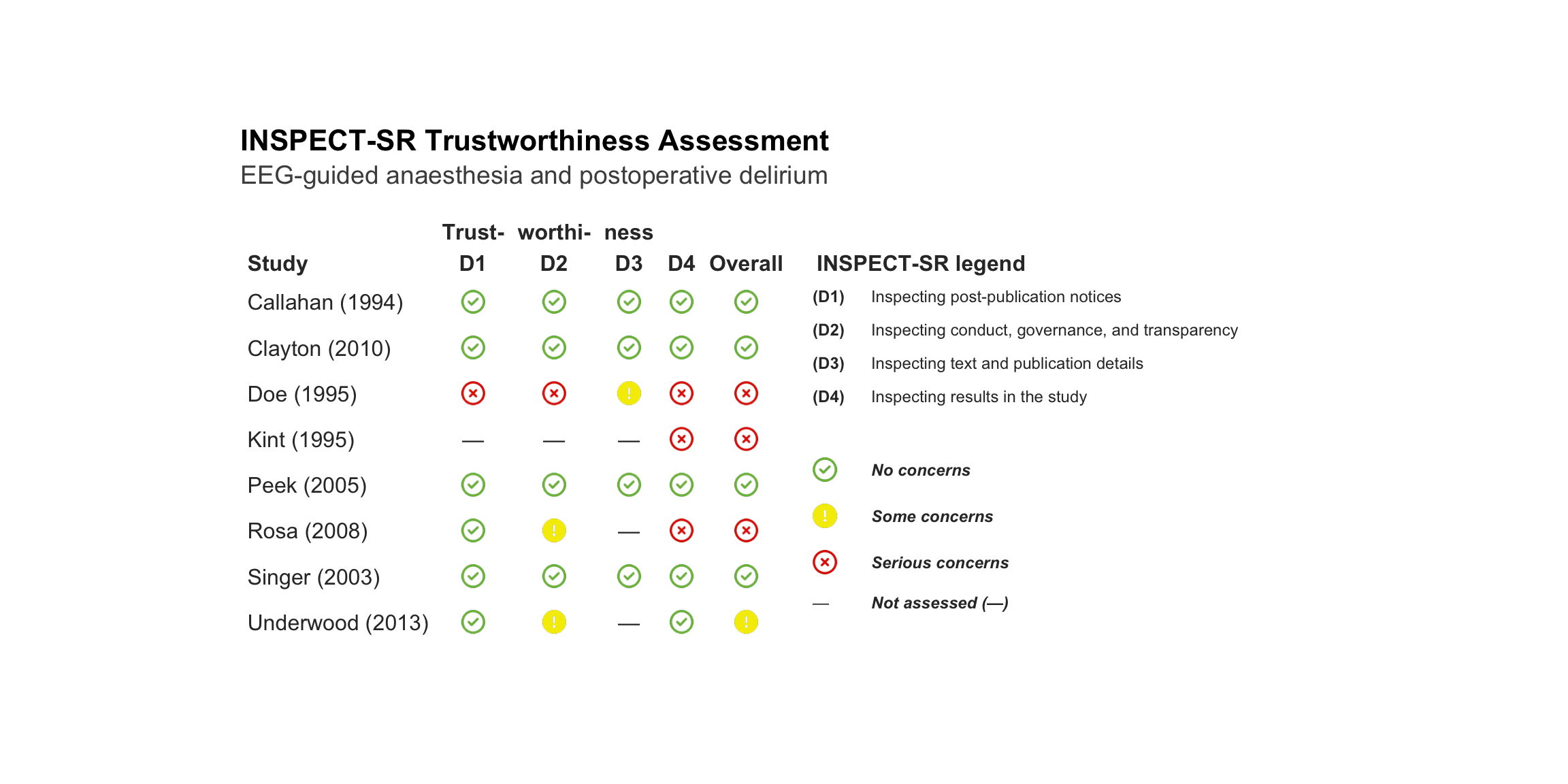
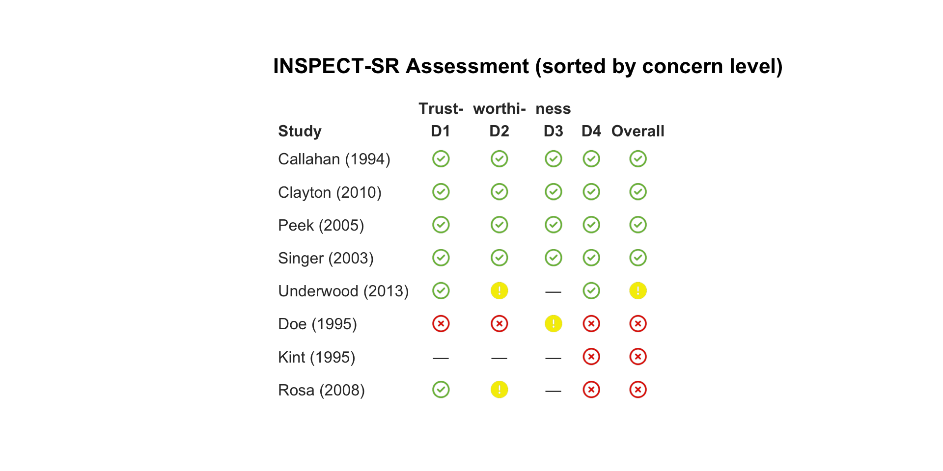
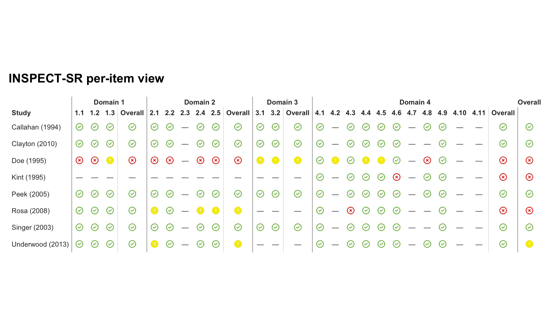
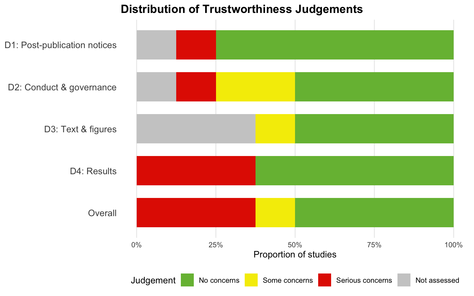
Skip to contents

Introduction

A systematic review is only as trustworthy as the primary studies it includes. Risk of bias tools assess whether a trial was conducted properly — they are not designed to detect whether the reported data are real.

INSPECT-SR (INveStigating ProblEmatic Clinical Trials in Systematic Reviews; Wilkinson et al., 2025) is a structured 21-item tool for assessing the trustworthiness of RCTs included in a systematic review. bayesma implements the full workflow in four steps:

  1. inspect_sr() — run the assessment (frequentist or Bayesian)
  2. inspect_sr_table() — inspect per-check details
  3. inspect_plot() / inspect_summary_plot() — visualise
  4. filter_trustworthy() — filter for meta-analysis

The four INSPECT-SR domains

Domain Items Focus
D1 3 Post-publication notices (retractions, expressions of concern)
D2 5 Conduct, governance, and transparency
D3 2 Text and publication details
D4 11 Results in the study (statistical anomalies)

Each domain receives No concerns, Some concerns, or Serious concerns. The overall judgement is the most severe domain. bayesma automates checks 4.3 (Carlisle), 4.6 (N consistency), 4.8 (GRIM), and 4.9 (p-value verification); the remaining 17 items are read from the input data frame.

The input data frame

inspect_sr() expects a single data frame with one row per study:

Column(s) Purpose
study Study identifier (required, unique)
n_randomised_int, n_randomised_ctrl, n_randomised_total, n_analysed_int, n_analysed_ctrl, n_lost_int, n_lost_ctrl CONSORT flow numbers → check 4.6
d1_1d4_11 Judgement for each item. Automated items (d4_3, d4_6, d4_8, d4_9) are overwritten
d1_1_commentd4_11_comment Optional free-text justification
baseline List-column of Table 1 data frames → GRIM (4.8) and Carlisle (4.3)
statistics List-column of reported test statistics → p-value check (4.9)
outcome_estimate, outcome_ci_lower, outcome_ci_upper, outcome_se, outcome_log_scale Optional primary outcome

Worked example

The package ships inspect_sr_example, an eight-trial simulated review:

Code
data(inspect_sr_example)

# One row per study — manual items as columns, variable-length data as list-columns
dplyr::glimpse(dplyr::select(inspect_sr_example, study, d1_1, d2_1, d3_1, d4_1))
Rows: 8
Columns: 5
$ study <chr> "Callahan (1994)", "Peek (2005)", "Clayton (2010)", "Singer (200…
$ d1_1  <chr> "No concerns", "No concerns", "No concerns", "No concerns", "No …
$ d2_1  <chr> "No concerns", "No concerns", "No concerns", "No concerns", "Som…
$ d3_1  <chr> "No concerns", "No concerns", "No concerns", "No concerns", NA, …
$ d4_1  <chr> "No concerns", "No concerns", "No concerns", "No concerns", "No …
Code
# Baseline data for the first study
inspect_sr_example$baseline[[1]]
   variable mean_int sd_int mean_ctrl sd_ctrl p_value integer_scale
1       Age     71.2    8.3      69.8     9.1    0.45         FALSE
2       BMI     24.8    4.1      25.1     3.9    0.72         FALSE
3 ASA_score      2.5    0.5       2.5     0.5    0.34          TRUE
Code
# Test statistics for a study with two tests
inspect_sr_example$statistics[[2]]
  test_type statistic  df df2 reported_p              context
1    chi_sq      4.12   1  NA       0.04   Delirium incidence
2         t     -0.85 437  NA       0.40 Duration of delirium

The eight trials span a range of profiles:

Study Expected
Callahan, Peek, Clayton, Singer Clean
Underwood Manual D2 “Some concerns” (late registration)
Rosa Carlisle flags too-perfect baseline balance
Doe Retracted; four GRIM failures
Kint CONSORT arithmetic inconsistency

Step 1 — inspect_sr()

Code
freq_results <- inspect_sr(inspect_sr_example, studyvar = study)

INSPECT-SR Trustworthiness Assessment
==================================================

Study                     D1    D2    D3    D4       Overall
----------------------------------------------------------------------
Callahan (1994)           OK    OK    OK    OK       No concerns
Peek (2005)               OK    OK    OK    OK       No concerns
Clayton (2010)            OK    OK    OK    OK       No concerns
Singer (2003)             OK    OK    OK    OK       No concerns
Underwood (2013)          OK    SOME  --    OK       Some concerns
Rosa (2008)               OK    SOME  --    SERIOUS  Serious concerns
Doe (1995)                SERIOUS SERIOUS SOME  SERIOUS  Serious concerns
Kint (1995)               --    --    --    SERIOUS  Serious concerns

Domains: D1 post-publication, D2 conduct/governance,
         D3 text/figures, D4 results (auto-filled for 4.3/4.6/4.8/4.9)
OK = No concerns, SOME = Some concerns, SERIOUS = Serious concerns
-- = Not assessed

For a per-check table, call inspect_sr_table().

The studyvar argument uses tidyeval (unquoted), consistent with bayesma() and bayes_forest().

Step 2 — inspect_sr_table()

Code
# All automated check details
inspect_sr_table(freq_results)
INSPECT-SR Automated Check Details
Domain 4 per-check results
Check Item Detail Result
Callahan (1994) Carlisle Baseline p-value distribution k = 3, fisher combined p = 0.3788, plausible Pass
GRIM ASA_score (Intervention) mean = 2.5, n = 46 Pass
ASA_score (Control) mean = 2.5, n = 46 Pass
N-consistency Total randomised = Intervention + Control expected = 92, observed = 92 Pass
Intervention: Randomised = Analysed + Lost expected = 46, observed = 46 Pass
Control: Randomised = Analysed + Lost expected = 46, observed = 46 Pass
Intervention: Lost <= Randomised expected = 46, observed = 3 Pass
Control: Lost <= Randomised expected = 46, observed = 2 Pass
P-value Delirium incidence reported p = 0.27, recalculated p = 0.2674 (diff 0.002593) Pass
Clayton (2010) Carlisle Baseline p-value distribution k = 3, fisher combined p = 0.46, plausible Pass
N-consistency Total randomised = Intervention + Control expected = 202, observed = 202 Pass
Intervention: Randomised = Analysed + Lost expected = 101, observed = 101 Pass
Control: Randomised = Analysed + Lost expected = 101, observed = 101 Pass
Intervention: Lost <= Randomised expected = 101, observed = 3 Pass
Control: Lost <= Randomised expected = 101, observed = 5 Pass
P-value Delirium incidence reported p = 0.1, recalculated p = 0.09545 (diff 0.004552) Pass
Doe (1995) Carlisle Baseline p-value distribution k = 4, fisher combined p = 0.05859, plausible Pass
GRIM ASA_score (Intervention) mean = 2.45, n = 90 Fail
ASA_score (Control) mean = 2.55, n = 90 Fail
Pain_VAS (Intervention) mean = 4.75, n = 90 Fail
Pain_VAS (Control) mean = 4.65, n = 90 Fail
N-consistency Total randomised = Intervention + Control expected = 180, observed = 180 Pass
Intervention: Randomised = Analysed + Lost expected = 90, observed = 90 Pass
Control: Randomised = Analysed + Lost expected = 90, observed = 90 Pass
Intervention: Lost <= Randomised expected = 90, observed = 2 Pass
Control: Lost <= Randomised expected = 90, observed = 3 Pass
P-value Delirium incidence reported p = 0.001, recalculated p = 0.000407 (diff 0.000593) Pass
Delirium duration reported p = 0.002, recalculated p = 0.001582 (diff 0.0004176) Pass
Kint (1995) Carlisle Baseline p-value distribution k = 3, fisher combined p = 0.4555, plausible Pass
GRIM Duration_surgery_min (Intervention) mean = 175, n = 150 Pass
Duration_surgery_min (Control) mean = 180, n = 150 Pass
N-consistency Total randomised = Intervention + Control expected = 300, observed = 300 Pass
Intervention: Randomised = Analysed + Lost expected = 150, observed = 147 Fail
Control: Randomised = Analysed + Lost expected = 150, observed = 146 Fail
Intervention: Lost <= Randomised expected = 150, observed = 5 Pass
Control: Lost <= Randomised expected = 150, observed = 8 Pass
P-value Delirium incidence reported p = 0.08, recalculated p = 0.07734 (diff 0.002663) Pass
Peek (2005) Carlisle Baseline p-value distribution k = 4, fisher combined p = 0.3872, plausible Pass
GRIM Duration_surgery_min (Intervention) mean = 185, n = 230 Pass
Duration_surgery_min (Control) mean = 190, n = 230 Pass
N-consistency Total randomised = Intervention + Control expected = 460, observed = 460 Pass
Intervention: Randomised = Analysed + Lost expected = 230, observed = 230 Pass
Control: Randomised = Analysed + Lost expected = 230, observed = 230 Pass
Intervention: Lost <= Randomised expected = 230, observed = 9 Pass
Control: Lost <= Randomised expected = 230, observed = 12 Pass
P-value Delirium incidence reported p = 0.04, recalculated p = 0.04238 (diff 0.002379) Pass
Duration of delirium reported p = 0.4, recalculated p = 0.3958 (diff 0.004209) Pass
Rosa (2008) Carlisle Baseline p-value distribution k = 6, fisher combined p = 4.265e-05, too_similar Fail
N-consistency Total randomised = Intervention + Control expected = 240, observed = 240 Pass
Intervention: Randomised = Analysed + Lost expected = 120, observed = 120 Pass
Control: Randomised = Analysed + Lost expected = 120, observed = 120 Pass
Intervention: Lost <= Randomised expected = 120, observed = 2 Pass
Control: Lost <= Randomised expected = 120, observed = 3 Pass
P-value Delirium incidence reported p = 0.005, recalculated p = 0.00511 (diff 0.0001103) Pass
Singer (2003) Carlisle Baseline p-value distribution k = 3, fisher combined p = 0.4289, plausible Pass
N-consistency Total randomised = Intervention + Control expected = 1232, observed = 1232 Pass
Intervention: Randomised = Analysed + Lost expected = 614, observed = 614 Pass
Control: Randomised = Analysed + Lost expected = 618, observed = 618 Pass
Intervention: Lost <= Randomised expected = 614, observed = 16 Pass
Control: Lost <= Randomised expected = 618, observed = 13 Pass
P-value Delirium incidence reported p = 0.67, recalculated p = 0.6714 (diff 0.001373) Pass
Underwood (2013) Carlisle Baseline p-value distribution k = 3, fisher combined p = 0.4773, plausible Pass
GRIM Duration_anaesthesia_min (Intervention) mean = 210, n = 80 Pass
Duration_anaesthesia_min (Control) mean = 198, n = 80 Pass
N-consistency Total randomised = Intervention + Control expected = 160, observed = 160 Pass
Intervention: Randomised = Analysed + Lost expected = 80, observed = 80 Pass
Control: Randomised = Analysed + Lost expected = 80, observed = 80 Pass
Intervention: Lost <= Randomised expected = 80, observed = 4 Pass
Control: Lost <= Randomised expected = 80, observed = 6 Pass
P-value Delirium incidence reported p = 0.02, recalculated p = 0.02506 (diff 0.005056) Pass
Code
# Only failures
inspect_sr_table(freq_results, only_failed = TRUE)
INSPECT-SR Automated Check Details
Domain 4 per-check results
Check Item Detail Result
Doe (1995) GRIM ASA_score (Intervention) mean = 2.45, n = 90 Fail
ASA_score (Control) mean = 2.55, n = 90 Fail
Pain_VAS (Intervention) mean = 4.75, n = 90 Fail
Pain_VAS (Control) mean = 4.65, n = 90 Fail
Kint (1995) N-consistency Intervention: Randomised = Analysed + Lost expected = 150, observed = 147 Fail
Control: Randomised = Analysed + Lost expected = 150, observed = 146 Fail
Rosa (2008) Carlisle Baseline p-value distribution k = 6, fisher combined p = 4.265e-05, too_similar Fail
Code
# Individual Tables
# E.g. Callaghan study
inspect_sr_table(freq_results, study = "Callaghan (1994)")
INSPECT-SR Automated Check Details
Domain 4 per-check results
Check Item Detail Result
Peek (2005) Carlisle Baseline p-value distribution k = 4, fisher combined p = 0.3872, plausible Pass
GRIM Duration_surgery_min (Intervention) mean = 185, n = 230 Pass
Duration_surgery_min (Control) mean = 190, n = 230 Pass
N-consistency Total randomised = Intervention + Control expected = 460, observed = 460 Pass
Intervention: Randomised = Analysed + Lost expected = 230, observed = 230 Pass
Control: Randomised = Analysed + Lost expected = 230, observed = 230 Pass
Intervention: Lost <= Randomised expected = 230, observed = 9 Pass
Control: Lost <= Randomised expected = 230, observed = 12 Pass
P-value Delirium incidence reported p = 0.04, recalculated p = 0.04238 (diff 0.002379) Pass
Duration of delirium reported p = 0.4, recalculated p = 0.3958 (diff 0.004209) Pass
INSPECT-SR Automated Check Details
Domain 4 per-check results
Check Item Detail Result
Clayton (2010) Carlisle Baseline p-value distribution k = 3, fisher combined p = 0.46, plausible Pass
N-consistency Total randomised = Intervention + Control expected = 202, observed = 202 Pass
Intervention: Randomised = Analysed + Lost expected = 101, observed = 101 Pass
Control: Randomised = Analysed + Lost expected = 101, observed = 101 Pass
Intervention: Lost <= Randomised expected = 101, observed = 3 Pass
Control: Lost <= Randomised expected = 101, observed = 5 Pass
P-value Delirium incidence reported p = 0.1, recalculated p = 0.09545 (diff 0.004552) Pass
INSPECT-SR Automated Check Details
Domain 4 per-check results
Check Item Detail Result
Singer (2003) Carlisle Baseline p-value distribution k = 3, fisher combined p = 0.4289, plausible Pass
N-consistency Total randomised = Intervention + Control expected = 1232, observed = 1232 Pass
Intervention: Randomised = Analysed + Lost expected = 614, observed = 614 Pass
Control: Randomised = Analysed + Lost expected = 618, observed = 618 Pass
Intervention: Lost <= Randomised expected = 614, observed = 16 Pass
Control: Lost <= Randomised expected = 618, observed = 13 Pass
P-value Delirium incidence reported p = 0.67, recalculated p = 0.6714 (diff 0.001373) Pass
INSPECT-SR Automated Check Details
Domain 4 per-check results
Check Item Detail Result
Underwood (2013) Carlisle Baseline p-value distribution k = 3, fisher combined p = 0.4773, plausible Pass
GRIM Duration_anaesthesia_min (Intervention) mean = 210, n = 80 Pass
Duration_anaesthesia_min (Control) mean = 198, n = 80 Pass
N-consistency Total randomised = Intervention + Control expected = 160, observed = 160 Pass
Intervention: Randomised = Analysed + Lost expected = 80, observed = 80 Pass
Control: Randomised = Analysed + Lost expected = 80, observed = 80 Pass
Intervention: Lost <= Randomised expected = 80, observed = 4 Pass
Control: Lost <= Randomised expected = 80, observed = 6 Pass
P-value Delirium incidence reported p = 0.02, recalculated p = 0.02506 (diff 0.005056) Pass
INSPECT-SR Automated Check Details
Domain 4 per-check results
Check Item Detail Result
Rosa (2008) Carlisle Baseline p-value distribution k = 6, fisher combined p = 4.265e-05, too_similar Fail
N-consistency Total randomised = Intervention + Control expected = 240, observed = 240 Pass
Intervention: Randomised = Analysed + Lost expected = 120, observed = 120 Pass
Control: Randomised = Analysed + Lost expected = 120, observed = 120 Pass
Intervention: Lost <= Randomised expected = 120, observed = 2 Pass
Control: Lost <= Randomised expected = 120, observed = 3 Pass
P-value Delirium incidence reported p = 0.005, recalculated p = 0.00511 (diff 0.0001103) Pass
INSPECT-SR Automated Check Details
Domain 4 per-check results
Check Item Detail Result
Doe (1995) Carlisle Baseline p-value distribution k = 4, fisher combined p = 0.05859, plausible Pass
GRIM ASA_score (Intervention) mean = 2.45, n = 90 Fail
ASA_score (Control) mean = 2.55, n = 90 Fail
Pain_VAS (Intervention) mean = 4.75, n = 90 Fail
Pain_VAS (Control) mean = 4.65, n = 90 Fail
N-consistency Total randomised = Intervention + Control expected = 180, observed = 180 Pass
Intervention: Randomised = Analysed + Lost expected = 90, observed = 90 Pass
Control: Randomised = Analysed + Lost expected = 90, observed = 90 Pass
Intervention: Lost <= Randomised expected = 90, observed = 2 Pass
Control: Lost <= Randomised expected = 90, observed = 3 Pass
P-value Delirium incidence reported p = 0.001, recalculated p = 0.000407 (diff 0.000593) Pass
Delirium duration reported p = 0.002, recalculated p = 0.001582 (diff 0.0004176) Pass
INSPECT-SR Automated Check Details
Domain 4 per-check results
Check Item Detail Result
Kint (1995) Carlisle Baseline p-value distribution k = 3, fisher combined p = 0.4555, plausible Pass
GRIM Duration_surgery_min (Intervention) mean = 175, n = 150 Pass
Duration_surgery_min (Control) mean = 180, n = 150 Pass
N-consistency Total randomised = Intervention + Control expected = 300, observed = 300 Pass
Intervention: Randomised = Analysed + Lost expected = 150, observed = 147 Fail
Control: Randomised = Analysed + Lost expected = 150, observed = 146 Fail
Intervention: Lost <= Randomised expected = 150, observed = 5 Pass
Control: Lost <= Randomised expected = 150, observed = 8 Pass
P-value Delirium incidence reported p = 0.08, recalculated p = 0.07734 (diff 0.002663) Pass

The table is grouped by study with thick separators. Failures are highlighted in red; passes in green.

Step 3 — Visualise

Traffic-light plot

Code
inspect_plot(
  freq_results,
  add_legend = TRUE,
  title    = "INSPECT-SR Trustworthiness Assessment",
  subtitle = "EEG-guided anaesthesia and postoperative delirium"
)

Sort by severity:

Code
inspect_plot(freq_results, sort_studies_by = "overall",
             title = "INSPECT-SR Assessment (sorted by concern level)")

Expanded per-item view

Set incl_checks = TRUE to see every INSPECT-SR item (1.1 … 4.11) grouped under domain spanner headers, with a per-domain Overall column and a final study-level Overall. The four Domain 4 cells filled in by the automated pipeline (4.3 Carlisle, 4.6 N-consistency, 4.8 GRIM, 4.9 p-value) appear alongside the manual items.

Code
inspect_plot(freq_results, incl_checks = TRUE,
             title = "INSPECT-SR per-item view")

Summary bar chart

Code
inspect_summary_plot(freq_results,
                     title = "Distribution of Trustworthiness Judgements")

Step 4 — Filter for meta-analysis

Code
# Primary analysis: exclude Serious concerns
data_primary <- filter_trustworthy(
  my_meta_data, freq_results,
  studyvar = study, exclude = "serious"
)

# Sensitivity: also exclude Some concerns
data_strict <- filter_trustworthy(
  my_meta_data, freq_results,
  studyvar = study, exclude = "some"
)

attr(data_primary, "excluded_studies")

The Bayesian extension

Pass bayes = TRUE to get Bayes factors instead of pass/fail:

Code
bayes_results <- inspect_sr(inspect_sr_example, studyvar = study, bayes = TRUE)

Bayesian INSPECT-SR Trustworthiness Assessment
======================================================================

Study                        Prior  Posterior         BF  Interpretation
------------------------------------------------------------------------------------------
Callahan (1994)              0.900      0.999      0.010  Trustworthy (no concerns)
Peek (2005)                  0.900      1.000      0.003  Trustworthy (no concerns)
Clayton (2010)               0.900      0.996      0.036  Trustworthy (no concerns)
Singer (2003)                0.900      0.995      0.049  Trustworthy (no concerns)
Underwood (2013)             0.900      0.999      0.011  Trustworthy (no concerns)
Rosa (2008)                  0.900      0.484      9.590  Likely untrustworthy (serious concerns)
Doe (1995)                   0.900      0.000        Inf  Likely untrustworthy (serious concerns)
Kint (1995)                  0.900      0.288     22.240  Likely untrustworthy (serious concerns)

BF: combined Bayes factor against trustworthiness (>1 = evidence against)
Posterior: P(trustworthy | data), prior = 0.9
>0.90 no concerns, 0.50-0.90 some concerns, <0.50 serious

The per-check BFs are visible in the table:

Code
inspect_sr_table(bayes_results, only_failed = TRUE)
INSPECT-SR Automated Check Details
Domain 4 per-check results
Check Item Detail Result BF
Doe (1995) Carlisle Baseline p-value distribution k = 4, fisher combined p = 0.05859, plausible Pass 2.04
GRIM ASA_score (Intervention) mean = 2.45, n = 90 Fail Inf
ASA_score (Control) mean = 2.55, n = 90 Fail Inf
Pain_VAS (Intervention) mean = 4.75, n = 90 Fail Inf
Pain_VAS (Control) mean = 4.65, n = 90 Fail Inf
Kint (1995) Carlisle Baseline p-value distribution k = 3, fisher combined p = 0.4555, plausible Pass 1.46
N-consistency Total randomised = Intervention + Control expected = 300, observed = 300 Pass 400.00
Intervention: Randomised = Analysed + Lost expected = 150, observed = 147 Fail 400.00
Control: Randomised = Analysed + Lost expected = 150, observed = 146 Fail 400.00
Intervention: Lost <= Randomised expected = 150, observed = 5 Pass 400.00
Control: Lost <= Randomised expected = 150, observed = 8 Pass 400.00
Peek (2005) Carlisle Baseline p-value distribution k = 4, fisher combined p = 0.3872, plausible Pass 1.65
Rosa (2008) Carlisle Baseline p-value distribution k = 6, fisher combined p = 4.265e-05, too_similar Fail 287.64
Singer (2003) Carlisle Baseline p-value distribution k = 3, fisher combined p = 0.4289, plausible Pass 1.42

Sensitivity to the prior

Code
r90 <- inspect_sr(inspect_sr_example, studyvar = study, bayes = TRUE,
                  prior_prob_trustworthy = 0.90, verbose = FALSE)
r75 <- inspect_sr(inspect_sr_example, studyvar = study, bayes = TRUE,
                  prior_prob_trustworthy = 0.75, verbose = FALSE)
r50 <- inspect_sr(inspect_sr_example, studyvar = study, bayes = TRUE,
                  prior_prob_trustworthy = 0.50, verbose = FALSE)

data.frame(
  Study   = r90$Study,
  Post_90 = round(r90$Posterior, 3),
  Post_75 = round(r75$Posterior, 3),
  Post_50 = round(r50$Posterior, 3)
)
             Study Post_90 Post_75 Post_50
1  Callahan (1994)   0.999   0.997   0.990
2      Peek (2005)   1.000   0.999   0.997
3   Clayton (2010)   0.996   0.988   0.965
4    Singer (2003)   0.995   0.984   0.953
5 Underwood (2013)   0.999   0.996   0.989
6      Rosa (2008)   0.484   0.238   0.094
7       Doe (1995)   0.000   0.000   0.000
8      Kint (1995)   0.288   0.119   0.043

The automated checks

GRIM test (check 4.8)

The mean of nn integer observations must equal k/nk/n for some integer kk. A reported mean that fails this is mathematically impossible.

Code
grim_test(3.45, n = 20)   # consistent
$consistent
[1] TRUE

$mean_value
[1] 3.45

$n
[1] 20

$decimals
[1] 2
Code
grim_test(3.47, n = 20)   # impossible
$consistent
[1] FALSE

$mean_value
[1] 3.47

$n
[1] 20

$decimals
[1] 2
Code
grim_test(2.45, n = 90)   # impossible (x.x5 at n=90)
$consistent
[1] FALSE

$mean_value
[1] 2.45

$n
[1] 90

$decimals
[1] 2

Bayesian version:

Code
bayes_grim_test(2.45, n = 90)
$bf_inconsistent
[1] Inf

$posterior_prob_inconsistent
[1] 1

$consistent_at_n
[1] FALSE

$consistent_nearby
[1] FALSE

$interpretation
[1] "strong_inconsistency"

$mean_value
[1] 2.45

$n
[1] 90

$decimals
[1] 2

P-value verification (check 4.9)

Code
verify_pvalue("chi_sq", statistic = 4.12, df = 1, reported_p = 0.04)
$consistent
[1] TRUE

$reported_p
[1] 0.04

$recalculated_p
[1] 0.04237908

$difference
[1] 0.002379078

$test_type
[1] "chi_sq"

$statistic
[1] 4.12
Code
verify_pvalue("chi_sq", statistic = 3.84, df = 1, reported_p = 0.004)
$consistent
[1] FALSE

$reported_p
[1] 0.004

$recalculated_p
[1] 0.05004352

$difference
[1] 0.04604352

$test_type
[1] "chi_sq"

$statistic
[1] 3.84

Carlisle’s test (check 4.3)

Code
carlisle_test(c(0.45, 0.12, 0.78, 0.33, 0.91))
$too_similar
[1] FALSE

$too_different
[1] FALSE

$combined_p
[1] 0.443096

$n_comparisons
[1] 5

$method
[1] "fisher"

$interpretation
[1] "plausible"
Code
carlisle_test(c(0.93, 0.81, 0.95, 0.94, 0.85, 0.95))
$too_similar
[1] TRUE

$too_different
[1] FALSE

$combined_p
[1] 4.264953e-05

$n_comparisons
[1] 6

$method
[1] "fisher"

$interpretation
[1] "too_similar"

Participant number consistency (check 4.6)

Code
check_n_consistency(
  n_randomised_int = 150, n_randomised_ctrl = 150,
  n_analysed_int = 142, n_analysed_ctrl = 138,
  n_lost_int = 5, n_lost_ctrl = 8
)
$consistent
[1] FALSE

$checks
                                       check expected observed  pass
1 Intervention: Randomised = Analysed + Lost      150      147 FALSE
2      Control: Randomised = Analysed + Lost      150      146 FALSE
3           Intervention: Lost <= Randomised      150        5  TRUE
4                Control: Lost <= Randomised      150        8  TRUE

$n_checks
[1] 4

$n_failed
[1] 2

Reporting

We assessed the trustworthiness of all included RCTs using INSPECT-SR (Wilkinson et al., 2025). Domain 4 checks were automated using the bayesma R package (GRIM test, p-value verification, Carlisle’s test, participant number consistency). Domains 1–3 were assessed manually by two independent reviewers. Studies with Serious concerns were excluded; Some concerns studies were retained in a sensitivity analysis.

References

Brown NJL, Heathers JAJ (2017). The GRIM test. Social Psychological and Personality Science, 8(4), 363–369.

Carlisle JB (2017). Data fabrication and other reasons for non-random sampling in 5,087 RCTs. Anaesthesia, 72(8), 944–952.

Wilkinson J, Heal C, Flemyng E, et al. (2025). INSPECT-SR: a tool for assessing trustworthiness of randomised controlled trials. BMJ, 389, e082938.